Deep Learning 习题一：Sparse Autoencoder

Deep Learning 练习一：Sparse Autoencoder

Step 1: Generate training set

The first step is to generate a training set. To get a single training example x, randomly pick one of the 10 images, then randomly sample an 8×8 image patch from the selected image, and convert the image patch (either in row-major order or column-major order; it doesn't matter) into a 64-dimensional vector to get a training example 

Complete the code in sampleIMAGES.m. Your code should sample 10000 image patches and concatenate them into a 64×10000 matrix.

To make sure your implementation is working, run the code in "Step 1" of train.m. This should result in a plot of a random sample of 200 patches from the dataset.

sampleIMAGES.m的代码：

106 or more examples, this will significantly slow down your code. Please implement sampleIMAGES so that you aren't making a copy of an entire 512×512 image each time you need to cut out an 8x8 image patch.
Step 2: Sparse autoencoder objective
Implement code to compute the sparse autoencoder cost function Jsparse(W,b) (Section 3 of the lecture notes) and the corresponding derivatives of Jsparse with respect to the different parameters. Use the sigmoid function for the activation function, . In particular, complete the code in sparseAutoencoderCost.m.
The sparse autoencoder is parameterized by matrices ,  vectors , . However, for subsequent notational convenience, we will "unroll" all of these parameters into a very long parameter vector θ with s1s2 + s2s3 +s2 + s3 elements. The code for converting between the (W(1),W(2),b(1),b(2)) and the θ parameterization is already provided in the starter code.
Implementational tip: The objective Jsparse(W,b) contains 3 terms, corresponding to the squared error term, the weight decay term, and the sparsity penalty. You're welcome to implement this however you want, but for ease of debugging, you might implement the cost function and derivative computation (backpropagation) only for the squared error term first (this corresponds to setting λ = β = 0), and implement the gradient checking method in the next section to first verify that this code is correct. Then only after you have verified that the objective and derivative calculations corresponding to the squared error term are working, add in code to compute the weight decay and sparsity penalty terms and their corresponding derivatives.
Step 3: Gradient checking
Following Section 2.3 of the lecture notes, implement code for gradient checking. Specifically, complete the code incomputeNumericalGradient.m. Please use EPSILON = 10-4 as described in the lecture notes.
We've also provided code in checkNumericalGradient.m for you to test your code. This code defines a simple quadratic function given by , and evaluates it at the point x = (4,10)T. It allows you to verify that your numerically evaluated gradient is very close to the true (analytically computed) gradient.
After using checkNumericalGradient.m to make sure your implementation is correct, next use computeNumericalGradient.m to make sure that yoursparseAutoencoderCost.m is computing derivatives correctly. For details, see Steps 3 in train.m. We strongly encourage you not to proceed to the next step until you've verified that your derivative computations are correct.
Implementational tip: If you are debugging your code, performing gradient checking on smaller models and smaller training sets (e.g., using only 10 training examples and 1-2 hidden units) may speed things up.
Step 4: Train the sparse autoencoder
Now that you have code that computes Jsparse and its derivatives, we're ready to minimize Jsparse with respect to its parameters, and thereby train our sparse autoencoder.
We will use the L-BFGS algorithm. This is provided to you in a function called minFunc (code provided by Mark Schmidt) included in the starter code. (For the purpose of this assignment, you only need to call minFunc with the default parameters. You do not need to know how L-BFGS works.) We have already provided code in train.m (Step 4) to call minFunc. The minFunc code assumes that the parameters to be optimized are a long parameter vector; so we will use the "θ" parameterization rather than the "(W(1),W(2),b(1),b(2))" parameterization when passing our parameters to it.
Train a sparse autoencoder with 64 input units, 25 hidden units, and 64 output units. In our starter code, we have provided a function for initializing the parameters. We initialize the biases  to zero, and the weights  to random numbers drawn uniformly from the interval , where nin is the fan-in (the number of inputs feeding into a node) and nout is the fan-in (the number of units that a node feeds into).
The values we provided for the various parameters (λ,β,ρ, etc.) should work, but feel free to play with different settings of the parameters as well.
Implementational tip: Once you have your backpropagation implementation correctly computing the derivatives (as verified using gradient checking in Step 3), when you are now using it with L-BFGS to optimize Jsparse(W,b), make sure you're not doing gradient-checking on every step. Backpropagation can be used to compute the derivatives of Jsparse(W,b) fairly efficiently, and if you were additionally computing the gradient numerically on every step, this would slow down your program significantly.

Step 5: Visualization
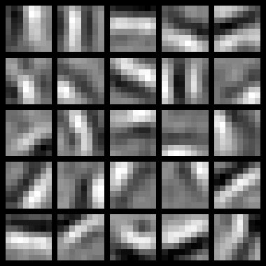
After training the autoencoder, use display_network.m to visualize the learned weights. (See train.m, Step 5.) Run "print -djpeg weights.jpg" to save the visualization to a file "weights.jpg" (which you will submit together with your code).
Results
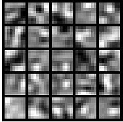
To successfully complete this assignment, you should demonstrate your sparse autoencoder algorithm learning a set of edge detectors. For example, this was the visualization we obtained:


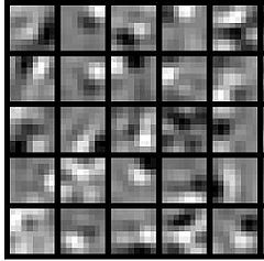
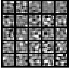
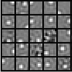
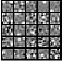
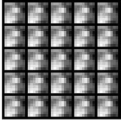
Our implementation took around 5 minutes to run on a fast computer. In case you end up needing to try out multiple implementations or different parameter values, be sure to budget enough time for debugging and to run the experiments you'll need.
Also, by way of comparison, here are some visualizations from implementations that we do not consider successful (either a buggy implementation, or where the parameters were poorly tuned):